
Activity 53.
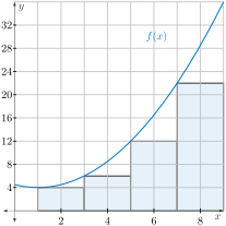
In Figure 189, rectangles have been drawn to approximate the area below \(y=f(x)\) and above the \(x\)-axis between \(x=1\) and \(x=9\) using a Riemann sum.
(a)
Calculate \(\Delta x\text{,}\) the width of each subinterval.
Answer.
\(\Delta x = 2\)
Solution.
\(\displaystyle \Delta x = \frac{9-1}{4} = 2\)
(b)
Does the diagram illustrate a left, right, or Midpoint Riemann sum? In the Riemann sum \(\displaystyle \sum_{k=1}^4 f(x_k^*) \Delta x\text{,}\) give an expression for \(x_k^*\) in terms of \(k\text{.}\) Then, calculate the value of the Riemann sum.
Answer.
This is a left Riemann sum whose value is \(88\text{.}\)
Solution.
This is a left Riemann sum. \(\displaystyle x_k^* = 1+2(k-1) = -1+2k\text{.}\) The value of the Riemann sum is \(\displaystyle \sum_{k=1}^4 f(x_k^*) \Delta x = 4(2) + 6(2) + 12(2) + 22(2) = 88\text{.}\)
(c)
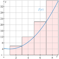
For \(\Delta x = 2\text{,}\) calculate the value of \(\displaystyle \sum_{k=1}^4 f(1+2k) \Delta x\) which also estimates this area. Then, illustrate the value or this Riemann sum with a figure similar to that shown in Figure 189.
Solution.
\begin{align*}
\displaystyle \sum_{k=1}^4 f(1+2k) \Delta x = \amp \mathstrut f(3)(2) + f(5)(2)+f(7)(2)+f(9)(2) \\
= \amp \mathstrut 6(2) + 12(2) + 22(2) + 36(2) \\
= \amp \mathstrut 152
\end{align*}
(d)
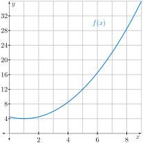
A better approximation is likely to come from a midpoint sum. Use sigma notation (as in (c)) to describe a midpoint Riemann sum with \(n=4\text{.}\) Use the sketch in Figure 191 as desired. Start by computing expressions for \(\Delta x\) and \(x_k^*\text{.}\)
Solution.
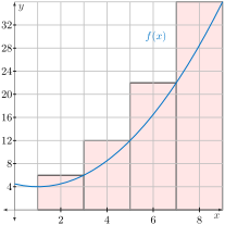
\(\Delta x = 2 \) and \(x_k^* = 2k\) so the midpoint Riemann sum is \(\displaystyle \sum_{k=1}^4 f(2k)(2)\)
(e)
What is the numerical value of the midpoint sum?
Answer.
Roughly \(4(2) + 8(2) + 16(2) + 28(2) = 112\text{.}\)

