Print preview

Handout Daily Prep 1.8 - The Tangent Line Approximation

Section Overview

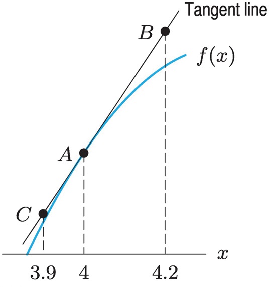
We are about to wrap up Chapter 1 of the text, titled “Understanding the Derivative.” One key aspect of understanding the derivative is how a differentiable function is locally linear. That is, how a differentiable function, up close, looks like a line. This enables us to use linear functions – the simplest functions in all of mathematics – as an effective tool to estimate the values of a differentiable function for $x$-values near a certain point where we know key information. Here, we are basically using some sophisticated ideas from calculus to do something natural: if we can see or identify a trend in how a function is changing at a given point, what might we predict for the future? Following a tangent line is a good approach to doing so.

Section Basic learning objectives

These are the tasks you should be able to perform with reasonable fluency when you arrive at our next class meeting. Important new vocabulary words are indicated in italics.

Given the value of the derivative of $f$ at a point $x=a$ (that is, given $f'(a)$), write the equation of the tangent line to the graph of $f$ at $x=a\text{.}$
Explain what is meant by the local linearization of a function $f$ at the point $x=a\text{.}$

Section To prepare for class

Complete all actions listed below. Respond to the questions highlighted with Submit.

Read motivating questions and the introduction to section 1.8 (up until the preview activity).
📝 [Submit] Do Preview Activity 1.8.1.
- (Optional) Watch video solution to Preview Activity 1.8.1 (3:11).
🔗
🔗
Watch the following video: Quick Review: The Tangent Line Approximation (2:16).
Explore the concept of local linearity through zooming! This applet, acting like a magnifying glass, illustrates this concept well. This second applet does it even better. Check both out.
Read section 1.8.2.
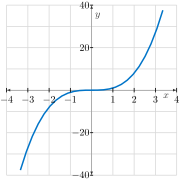
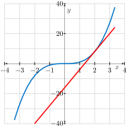
📝 [Submit] Watch this video on Calculating a Tangent Line. Then, use the local linearization to estimate the value of $f(-2.1)$ for the example presented.
Read section 1.8.3.
📝 [Submit] Re-read Example 1.8.2. Then, write two sentences about the use of the word near in this context. How near is near? How might near depend on the function?
Watch this video on estimating functional values: Using a Tangent Line (3:26).
Watch this video on using the local linearization: Using the Local Linearization (7:06).
Do these problems.
1. Determine the equation of the tangent line to $y=x^{3}$ at $x=2\text{.}$ Sketch this tangent line on the curve to verify its reasonableness.
  
  $A coordinate graph showing a single smooth curve. The curve increases from left to right, starting in the lower left and ending in the upper right. It passes near the origin and flattens slightly around x equals 0 before increasing more steeply for positive x. The x- and y-axes are labeled, with tick marks extending from approximately minus 40 to 40 on the y-axis and minus 4 to 4 on the x-axis.$
  
  Figure 48. The graph of $y=x^3\text{.}$
2. The graph of the function shown in Figure 49 has $f(4)=220$ and $f'(4) = 15\text{.}$
  1. Estimate the value of $f(3.9)\text{.}$
  2. Find the coordinates of the points $A\text{,}$ $B\text{,}$ and $C\text{.}$
  🔗
  Figure 49.
  
  🔗
🔗
🔗
Ask Copilot “Are all functions $f(x)$ locally linear? If not, give me an example.”
Ask Copilot “What is the relationship between local linearity and tangent lines for functions of a single variable?”

Checkpoint 50. When Is a Tangent Line Approximation Useful?

Sort each statement according to the idea it best illustrates.

Estimate $\sqrt{4.1}$ using information about $\sqrt{x}$ at $x=4\text{.}$
Approximate a function value at an input close to a known point.
Tangent line approximation is likely to work well.
Estimate $\sqrt{100}$ using the tangent line to $\sqrt{x}$ at $x=4\text{.}$
Use local information many units away from the point of tangency.
Tangent line approximation is likely to work poorly.
Zooming in near a differentiable point makes the graph look almost linear.
The tangent line closely resembles the function nearby.
Local linearity.

Section After class

Solidifying the concepts discussed in class through practice is necessary to build your skills.

Do Exercises 1-6 in section 1.8.5.
Do written exercises 7-10 in section 1.8.5.
Explore applet demonstrating $\displaystyle \lim_{\theta \rightarrow 0}\frac{\sin \theta}{\theta}$. Though this is not critical knowledge, and is a bit complicated, this proves a very important limit: $\displaystyle \lim_{\theta \rightarrow 0}\frac{\sin \theta}{\theta}= 1\text{.}$
Start working on the MOMwork (MyOpenMath) assignment for this section.

Section Advanced learning objectives

In addition to mastering the basic objectives, here are the tasks you should be able to perform after class, with practice:

Compute the linear approximation of a function at a specific point.
Use the linear approximation/local linearization of a function at $x=a$ to approximate values of $f$ near $x=a\text{.}$
Use the second-order derivative to determine whether an approximation is an overestimate or an underestimate. (If $L(x)$ is the local linearization of a function $f(x)$ at $x=a\text{,}$ and if $b$ is some point near $a\text{,}$ determine whether $L(b)$ is greater than, less than, or equal to $f(b)$ and explain.)
Describe how the concept of local linearity gives $\displaystyle \lim_{\theta \rightarrow 0}\frac{\sin \theta}{\theta}=1\text{.}$

Section Additional suggestions

Watch the following video comparing secant to tangent lines: Slopes of Secant and Tangent Lines - Part I (6:26).
Watch this video which will reinforce idea of using a tangent line: Slopes of Secant and Tangent Lines - Part 2 (6:52).
Watch this video (4:11) if you just want to see another (basic) example of finding the local linearization of a function at a point.

Section Answers

The slope of the tangent line at $x=2$ is 12. The equation of the tangent line is $y=12x-16\text{.}$

$A coordinate graph showing a smooth blue curve and a straight red line. The blue curve increases from left to right, passing near the origin, flattening slightly around x equals 0, and then rising more steeply for positive x. The red line has constant positive slope, intersects the y-axis below zero, and crosses the blue curve near x equals 2. The x- and y-axes are labeled, with tick marks extending from approximately minus 4 to 4 on the x-axis and minus 40 to 40 on the y-axis.$

Figure 51. The graph of $y=x^3$ and its tangent line at $x=2\text{.}$
1. $\displaystyle f(3.9) \approx 218.5$
2. $A$ has coordinates $(4,220)\text{;}$ $B$ has coordinates $(4.2,223)\text{;}$ $C$ has coordinates $(3.9,218.5)$
🔗
🔗

Prev Top Next