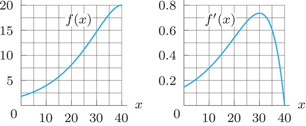
Functions are a powerful tool in mathematics: each describes a rule or process that takes any valid input to one and only one output. One of the natural questions that arises regarding any function is “can the rule be undone (or reversed)?” Indeed, this is connected to the concept of a function’s inverse. While not every function has an inverse, for those that do, knowing the inverse can be valuable in a wide range of settings.
Among the most important inverse functions in mathematics are the natural logarithm function, \(\ln(x)\) (which is the inverse of the exponential function, \(e^{x}\)) and the inverse trigonometric functions, such as \(\arcsin(x)\) and \(\arctan(x)\text{.}\)
In this section of the text, we explore how we can use the relationship between a function and its inverse to determine the derivative formula for the inverse function and, along the way, learn a key geometric connection between a function’s derivative and the derivative of its inverse.
These are the tasks you should be able to perform with reasonable fluency when you arrive at our next class meeting. Important new vocabulary words are indicated in italics.
📝 [Submit] Do the following to construct the function \(\log_{2}(x)\) (the inverse of the exponential function \(2^{x}\)) in GeoGebra. Submit screenshots as needed.
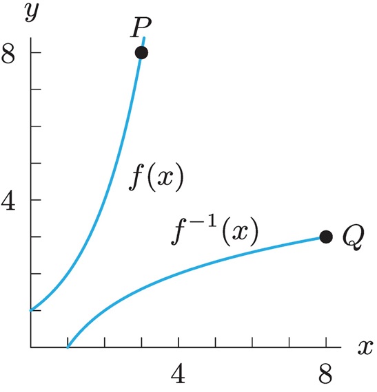
We now sketch a diagonal line about which we will reflect. The third box on the menu offers the option Lines. Choose it and then point to the origin \((0,0)\) and click to place point \(A\) and then point to \((1,1)\) and click to place point \(B\text{.}\) A line will be constructed through these two points. Remember that two points determine a line. [Yes, this is the line \(y=x\text{.}\)]
We are now ready to reflect the graph of \(f(x)\) about this line. GeoGebra has a built-in tool to do this. Select the ninth box on the menu and the option Reflect about line. Choose it. Then, click on the graph of \(2^{x}\) to select it. Second, click on the line \(y=x\) to select it. The reflection of the graph of \(y=2^{x}\) should appear.
To complete our replication of Figure 2.6.2 in the text, let’s plot the point \(\displaystyle (-1,\frac{1}{2})\text{.}\) In the next input box, type C = (-1,f(-1)). The point \(\displaystyle (-1,\frac{1}{2})\) will be plotted on your graph of \(f(x)\text{.}\) Repeat the process used to reflect the graph about the line \(y=x\) to reflect the point\(C\) about this same line: From the menu, select Reflect about line, then select point C on the graph and finally select the line \(y=x\text{.}\) A new point on the graph of the inverse of \(2^{x}\) should appear at \(\displaystyle (\frac{1}{2}, -1)\text{.}\)
To verify that you have indeed found the graph of \(\log_{2}(x)\text{,}\) type log2(x) in the next input box. GeoGebra will plot this function right on top of your reflection if you have followed this procedure correctly.
Let’s try this for a second function. Delete the graph of \(\log_{2}(x)\text{.}\) Then, go to the first input box and change 2\(\wedge\)x to sqrt(x). Your output should be automatically updated. Does it look correct? How do you know?
Do the following problem. Use the graph of \(2^{x}\) and the graph of \(\log_{2}(x)\) found during your GeoGebra construction if you wish. [Note: The co-domain is defined in the reading.]
📝 [Submit] Watch video Examples of Derivatives with the Natural Log (6:29). In this video, the chain rule is used to take a derivative of a composite function of the form \(f(g(x))\text{.}\) Identify \(g(x)\text{,}\)\(f(x)\text{,}\)\(g'(x)\) and \(f'(x)\) for that example.
Match each piece of information about \(f\) with the corresponding value of the derivative of its inverse. Recall that if \(f(a)=b\text{,}\) then \((f^{-1})'(b)=\dfrac{1}{f'(a)}\text{.}\)
Explore an applet Derivatives of Inverse Functions to better understand the steps involved in the process of finding the derivative of an inverse function. Be sure to read the Explore questions for each step on the slider.
Use the relationship between a function and its inverse to develop the inverse function’s derivative rule (in particular: be able to do this “from scratch” for \(\ln(x)\text{,}\)\(\arcsin(x)\text{,}\) and \(\arctan(x)\)).
Differentiate a function involving logarithmic functions, arcsine and arctangent functions, and for which the derivative involves a combination of chain, product and quotient rules.