
Print preview
Handout Daily Prep 4.3 - The Definite Integral
Section Overview
In this section we introduce a notation used for expressing the limit of a Riemann sum. We thus define what a definite integral is. We will be discussing the definition, meaning, and use of the definite integral for the remainder of the course. Surprisingly, it has a very strong and natural connection to the derivative – a connection we will discuss and explore in Section 4.4. However, in this section, we deduce the properties that this new mathematical object, the definite integral, has based on its definition and its geometrical interpretation.
Section Basic learning objectives
These are the tasks you should be able to perform with reasonable fluency when you arrive at our next class meeting. Important new vocabulary words are indicated in italics.
-
Recognize the parts of the limit definition of the definite integral, especially how the definite integral results from taking a limit of Riemann sums.
-
Identify an integral sign, integrand, and limits of integration.
-
Explain what it means to evaluate a definite integral.
-
Interpret, geometrically, the quantity denoted by \(\displaystyle \int_{a}^{b} f(x) \ dx\text{.}\)
-
Recognize and apply properties that the definite integral possesses. Use these properties to evaluate definite integrals in special circumstances.
Section To prepare for class
Complete all actions listed below. Respond to the questions highlighted with Submit.
-
Read motivating questions and the introduction to section 4.3 (up until Preview Activity 4.3.1).
-
📝 [Submit] Do Preview Activity 4.3.1.
-
Watch video Quick Review - The Definite Integral (3:00).
-
Read section 4.3.2 up to Activity 4.3.2.
-
📝 [Submit] Explore the applet Gaining Geometric Intuition. Submit answers to questions #3-6 at the bottom of the webpage.
-
Prompt Copilot “Please produce and execute Python code that illustrates an upper Riemann sum of the function \(f(x)=\cos(x)+1\) from \(x=0\) to \(x=3\pi\) using n=10 rectangles.”
-
Do these problems.
-
-
Use geometry to evaluate \(\displaystyle \int_{-1}^{4} 1-\frac{1}{2}x \ dx\text{.}\)
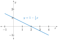
Figure 116. The graph of \(y=1-\frac{1}{2}x\) can be used to evaluate \(\displaystyle \int_{-1}^4 1-\frac{1}{2}x \ dx\text{.}\) -
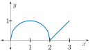
Figure 117.
-
-
Use Table 118 to estimate \(\displaystyle \int_{0}^{12}f(x) \ dx\text{.}\) Find a left sum \(L_{4}\text{,}\) a right sum \(R_{4}\text{,}\) and then average the two.
Table 118. Values of \(f\) on \([0,12]\text{.}\) \(x\) 0 3 6 9 12 \(f(x)\) 20 10 5 2 1 -
Figure 119 illustrates Riemann sum approximations, \(\displaystyle \sum_{k=1}^{n} f(x_{k}^{*}) \Delta x_{k}\text{,}\) to \(\displaystyle \int_{a}^{b} f(x) \ dx\text{.}\) In each, determine the values of \(a, b\text{,}\) and \(n\text{.}\) Then, give expressions for \(\Delta x_{k}\) and \(x_{k}^{*}\text{.}\)
![Graph of a decreasing function f(x) on the interval from x = 1 to x = 4. A blue curve slopes downward as x increases. Three left-endpoint rectangles are drawn under the curve, each shaded in light blue, with widths spanning the intervals [1, 2], [2, 3], and [3, 4]. The heights of the rectangles are determined by the function values at x = 1, 2, and 3. Axes are labeled x and y.](generated/latex-image/FindXstar1.svg)
![Graph of a decreasing function f(x) on the interval from x = 1 to x = 4. The blue curve slopes downward as x increases. Five left‑endpoint rectangles are drawn under the curve, each shaded in light blue. The heights of the rectangles decrease across the intervals [1, 1.6], [1.6, 2.2], [2.2, 2.8], [2.8, 3.4], and [3.4, 4]. Axes are labeled x and y. The rectangles form a left‑endpoint Riemann sum approximation of the area under the curve.](generated/latex-image/FindXstar2.svg)
Figure 119. Riemann sum approximations of \(\int_a^b f(x) \ dx\text{.}\)
-
-
Prompt Copilot “Please produce and execute Python code that illustrates a middle Riemann sum of the function f(x)=x\(\wedge\)2+1 from x=1 to x=3 using n=5 rectangles.” Does the AI give you a correct value for the sum being illustrated?
-
Read section 4.3.3 on properties of the definite integral.
Section After class
Solidifying the concepts discussed in class through practice is necessary to build your skills.
-
Read section 4.3.4.
-
Watch video Average Value of a Function (7:34).
-
Explore a nice visualization of The Average Value of a Function.
-
Explore the Average Value of a Linear Function geometrically.
-
Read section 4.3.5 - summary.
-
Start working on the MOMwork (MyOpenMath) assignment for this section.
Section Advanced learning objectives
In addition to mastering the basic objectives, here are the tasks you should be able to perform after class, with practice:
-
Compute the average value of a function on the interval \([a,b]\) using \(\displaystyle \int_{a}^{b} f(x) \ dx\text{.}\)
-
Interpret the average value of a function as the height of a rectangle.
Section Additional suggestions
-
Watch video Riemann Sum Notation (2:04).
-
Watch video Riemann Sums - How to use Sigma Notation (6:33).
-
Finish (if needed) Activity 4.3.2.
-
(Optional) Watch video explaining parts (a)-(c) of Activity 4.3.2 (4:00).
-
(Optional) Watch video explaining part (d) of Activity 4.3.2 (2:47).
-
-
Watch video Average Value of a Function with an Integral (2:09).
-
Explore another way to visualize the Average Value of a Function.
-
Explore three more applets illustrating the average value of a function.
-
Do these problems.
-
Suppose \(f(x)\) is an odd function (as shown in Figure 121) with \(\displaystyle \int_{-2}^{0} f(x) \ dx = 4\text{.}\)
-
Evaluate \(\displaystyle \int_{0}^{2} f(x) \ dx\)
-
Evaluate \(\displaystyle \int_{-2}^{2} f(x) \ dx\)
-
Evaluate \(\displaystyle \int_{-2}^{2} |f(x)| \ dx\)
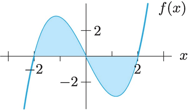
Figure 121. -
-
Consider approximating the definite integral \(\displaystyle \int_{0.5}^{5} \frac{4}{1+x}\ dx\) by a Riemann sum approximation\begin{equation*} \sum_{k=1}^{3} \frac{4}{1+\left[ 0.5+k \cdot \left( \frac{3}{2}\right)\right]}\cdot \left( \frac{3}{2}\right). \end{equation*}Using Figure 122, carefully illustrate this Riemann sum as in the last problem. Is this a left sum, a right sum, or neither? Evaluate this sum.
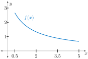
Figure 122. -
Using sigma (\(\Sigma\)) notation, give a middle sum Riemann approximation with \(n=3\) (see Figure 123) that estimates the value of the definite integral \(\displaystyle \int_{0.5}^{5} \frac{4}{1+x}\ dx\text{.}\) Hint: The previous problem can serve as a guide.
![Graph of a decreasing function f(x) on the interval from x = 1 to x = 5. The curve begins above y = 2 near x = 1 and slopes downward toward y = 1 by x = 5. Four left‑endpoint rectangles are drawn under the curve, each shaded in light blue, spanning the intervals [1, 2], [2, 3], [3, 4], and [4, 5]. The heights of the rectangles decrease from left to right, forming a left‑endpoint Riemann sum approximation of the area under the curve.](generated/latex-image/IntegralMiddleSumApproxPic.svg)
Figure 123. A middle sum approximation with \(n=3\text{.}\)
-
-
Watch video What Definite Integrals Are (6:38).
-
Watch video Definite Integrals and Riemann Sums (3:51).
-
Do these problems.
-
Suppose that \(C(t)\) represents the daily cost of heating your house, measured in dollars per day, where \(t\) is the time measured in days and \(t=0\) corresponds to January 1, 2020. Interpret \(\displaystyle \int_{0}^{90}C(t) \ dt\) and \(\displaystyle \frac{1}{90-0}\int_{0}^{90}C(t) \ dt\text{.}\)
-
The value, \(V\text{,}\) of a Tiffany lamp, worth $225 in 1975, increases at 15% per year. Its value in dollars \(t\) years after 1975 is given by \(V = 225(1.15)^{t}\text{.}\) Find the average value of the lamp over the period 1975-2015. The Average Value of a Function applet produces a nice way to calculate this. Hint: Hold the SHIFT key to stretch each axis pictures as needed. Stretch the vertical axis, for example, to about 70,000.
-
Section Answers
Subsection To prepare for class
-
-
\(\displaystyle \displaystyle \frac{5}{4}\)
-
\(\displaystyle \displaystyle \frac{\pi+1}{2}\)
-
-
\(L_{4} = (20)(3) + (10)(3) + (5)(3) + (2)(3) = 111, R_{4} = 54\text{;}\) these average to 82.5.
-
-
\(\displaystyle \displaystyle a=1, b=4, n=3, \Delta x_{k} = 1, x_{k}^{*} = k+\frac{3}{4}\)
-
\(\displaystyle \displaystyle a=0.5, b=3.5, n=6, \Delta x_{k} = 0.5, x_{k}^{*} = \frac{1}{2}k\)
-
Subsection Additional suggestions
-
-
-4
-
0
-
8
-
-
This is a right sum \(R_{3}\text{.}\)Here, \(\displaystyle a=0.5, b=5, n=3, \Delta x_{k} = \frac{3}{2}\) and\(\displaystyle x_{k}^{*} = \frac{1}{2}+ k\left(\frac{3}{2}\right)\text{.}\) The sum is\(\displaystyle \frac{4}{1+2}(1.5) + \frac{4}{1+3.5}(1.5) + \frac{4}{1+5}(1.5) = 4.\overline{3}\text{.}\)
-
Here \(\displaystyle \Delta x_{k} = \frac{6}{4}\text{,}\) \(\displaystyle x_{k}^{*} = -\frac{1}{4}+ k\left(\frac{6}{4}\right)\text{.}\)So, \(\displaystyle \sum_{k=1}^{3}\frac{4}{1+\left[ -\frac{1}{4}+k\left(\frac{6}{4}\right) \right]}\cdot \left(\frac{6}{4}\right)\text{.}\)
Subsection And yet additional suggestions
-
\(\displaystyle \int_{0}^{90}C(t) \ dt\) represents the total cost to heat house for the first 90 days of 2020 (in dollars).\(\displaystyle \frac{1}{90-0}\int_{0}^{90}C(t) \ dt\) represents the average cost (dollars per day) of heating the house for the first 90 days of 2020.
-
\(\displaystyle \frac{1}{40-0}\int_{0}^{40}V(t) \ dt = \frac{1}{40}\int_{0}^{40}225(1.15)^{t} \ dt \approx \$10,740.46\text{.}\) The Average Value of a Function applet produces a nice way to see this as illustrated in Figure 124.
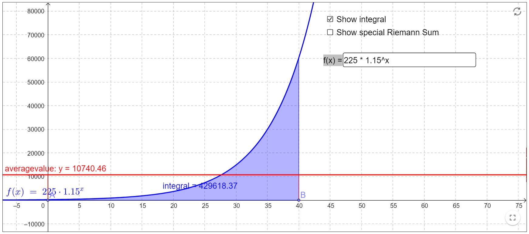
Figure 124. The average value of \(y=225(1.15)^x\) on \([0,40]\text{.}\)

