Print preview

Handout Daily Prep 1.7 - Limits, Continuity, and Differentiability

Section Overview

We are returning to study limits of general functions, and examine how we can evaluate them. In particular, we will see that functions which are “nice” in a certain way (we will call such functions “continuous”) allow us to evaluate limits very easily. Knowing which functions are continuous or where they fail to be continuous will then enable us to focus on the interesting parts of functions, where we actually need to consider a limit.

We are about to wrap up Chapter 1 of the text, titled Understanding the Derivative. One key aspect of understanding the derivative is how a differentiable function is locally linear. That is, how a differentiable function, up close, looks like a line. This enables us to use linear functions – the simplest functions in all of mathematics – as an effective tool to estimate the values of a differentiable function for x-values near a certain point where we know key information. Here, we are basically using some sophisticated ideas from calculus to do something natural: if we can see or identify a trend in how a function is changing at a given point, what might we predict for the future? Following a tangent line is a good approach to doing so.

This section covers the following concepts: Limit Laws and how to use them to evaluate limits algebraically, One-sided limits, Continuity, Direct Substitution Property, Evaluating (one-sided) limits algebraically, Differentiability, Relationship between Differentiability and Continuity, Linearization of a function.

Section Basic learning objectives

These are the tasks you should be able to perform with reasonable fluency when you arrive at our next class meeting. Important new vocabulary words are indicated in italics.

Describe left-handed and right-handed limits.
Describe the difference between a limit and a one-sided limit.
Estimate a limit from the left and from the right of a function at a point on a graph (or determine that it does not exist).
State the definition of a continuous function $f$ at a point $x=a$ and on an interval $[a,b]\text{.}$
Determine whether a function is continuous at a point by examining the graph of that function.
State informally what it means for a function to be differentiable at a point (use the expression locally linear).
Determine whether a function is differentiable at a point by examining the graph of that function.
Provide examples of functions that are continuous and yet not differentiable at a specific point.

Section To prepare for class

Complete all actions listed below. Respond to the questions highlighted with Submit.

Read motivating questions and the introduction to section 1.7 (up until the preview activity).
Do Preview Activity 1.7.1.
- (Optional) Watch video solution to Preview Activity 1.7.1 (6:25).
🔗
🔗
Watch video: Quick Review: Limits, Continuity, and Differentiability (4:01).
Read section 1.7.2 (up until Activity 1.7.2).
📝 [Submit] Explore the graphical idea of a limit with this applet. Investigate the limit as $x$ approach -4, as $x$ approaches -1, and as $x$ approaches 2.
Watch this video that speaks more precisely as to how a limit is truly defined: Limit at a Point (7:15).
Watch this video on one-sided limits: One-sided Limits (7:23).
Read section 1.7.3 (up until Activity 1.7.3).
📝 [Submit] Re-read Definition 1.7.4 in the text. Then, give an example of a function that
- satisfies (a) but not (b).
- satisfies (b) but not (a).
- satisfies (a) and (b), but not (c).
🔗
🔗
Watch this video on continuity at a point: Determining Continuity (7:21).
Watch three videos on the subject of continuity: Definition of Continuity (3:36), Removable Discontinuities (7:13), and Continuous Functions (2:38).
Do these exercises.
1. Explore this Desmos applet answering the following questions.
  1. Without making any adjustments to the Desmos graph, determine the numerical value of the limit at $x=7\text{.}$
  2. Without making any adjustments to the Desmos graph, determine the value of the function at $x=7\text{.}$
  3. By using the slider for $x_{0}$ or dragging the red point currently located at $(5,2)\text{,}$ explore the graph as $x$ increases from 5 to 8. Is the function continuous at $x=7\text{?}$
  4. Now, drag the blue point currently located at $(7,3)$ to $(7,1)\text{.}$ You may also use the numerical slider for $b\text{.}$
    After making this adjustment to the Desmos graph, determine the numerical value of the limit at $x=7\text{.}$
    
    After making this adjustment to the Desmos graph, determine the value of the function at $x=7\text{.}$
    
    By using the slider for $x_{0}$ or dragging the red point currently located at $(5,2)\text{,}$ explore the graph as $x$ increases from 5 to 8. Is the function continuous at $x=7\text{?}$
    🔗
  5. Now, drag the blue point currently located at $(3,2)$ to $(3,1)\text{.}$ You may also use the numerical slider for $a\text{.}$
    After making this adjustment to the Desmos graph, determine the value of the limit at $x=3$ from the left.
    
    After making this adjustment to the Desmos graph, determine the value of the limit at $x=3$ from the right.
    
    After making this adjustment to the Desmos graph, determine the value of the function at $x=3\text{.}$
    
    By using the slider for $x_{0}$ or dragging the red point currently located at $(5,2)\text{,}$ explore the graph as $x$ decreases from 5 to 2. Which of the following is true about the function at $x=3\text{?}$ [Continuous from the left OR Continuous from the right OR Continuous]
    🔗
  6. Now, drag the blue point currently located at $(3,2)$ to $(3,4)\text{.}$ You may also use the numerical slider for $a\text{.}$
    After making this adjustment to the Desmos graph, determine the value of the limit at $x=3$ from the left.
    
    After making this adjustment to the Desmos graph, determine the value of the limit at $x=3$ from the right.
    
    After making this adjustment to the Desmos graph, determine the value of the function at $x=3\text{.}$
    
    By using the slider for $x_{0}$ or dragging the red point currently located at $(5,2)\text{,}$ explore the graph as $x$ decreases from 5 to 2. Which of the following is true about the function at $x=3\text{?}$ [Continuous from the left OR Continuous from the right OR Continuous]
    🔗
  7. A discontinuity is removable if the function can be made continuous at the point by changing the function value.
    Is the discontinuity at $x=3$ a removable discontinuity?
    
    Is the discontinuity at $x=7$ a removable discontinuity?
    🔗
  🔗
  📝 [Submit] Now answer these questions.
  - Write what you believe is the purpose of this particular exercise. That is, what did you learn from doing this problem?
  - This entire section of the text might have been titled Smoothness. In a sentence or two, how does this word relate to the topics in this section?
  🔗
  🔗
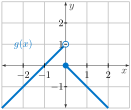
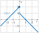
2. The graphs of functions $f$ and $g$ are given in Figure 42.
  
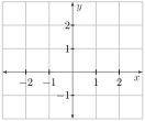
  $Three side-by-side coordinate graphs. Left: a piecewise linear graph labeled g(x). For x less than zero, a rising line approaches an open circle at (0, 1). For x greater than or equal to zero, a descending line begins at a filled point at (0, 0). Middle: a piecewise linear graph labeled f(x). For x less than or equal to zero, a rising line ends at a filled point at (0, 2). For x greater than zero, a descending line begins at an open circle at (0, 1). Right: a blank coordinate grid with labeled x- and y-axes.$
  
  Figure 42. A limit question involving two piecewise-defined functions.
  1. Plot $(f-g)(x) = f(x)-g(x)$ using the empty grid.
  2. Does $\displaystyle \lim_{x \rightarrow 0^-}f(x) - \lim_{x \rightarrow 0^-}g(x) = \lim_{x \rightarrow 0^-}[f(x)-g(x)]\text{?}$
  3. Does $\displaystyle \lim_{x \rightarrow 0^+}f(x) - \lim_{x \rightarrow 0^+}g(x) = \lim_{x \rightarrow 0^+}[f(x)-g(x)]\text{?}$
  4. Does $\displaystyle \lim_{x \rightarrow 0}f(x) - \lim_{x \rightarrow 0}g(x) = \lim_{x \rightarrow 0}[f(x)-g(x)]\text{?}$
  🔗
  🔗
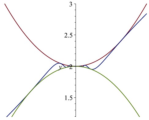
3. The graph of the function $\displaystyle f(x) = 2+x^{2} \sin(1/x)$ is sandwiched between the graphs of $g(x) = 2-x^{2}$ below and $h(x) = 2+x^{2}$ above. Compute the value of $\displaystyle \lim_{x \rightarrow 0}\left( 2+x^{2} \sin(1/x) \right)\text{.}$ Defend your answer.
  
  Figure 43. A function $f(x)=2+x^2\sin(1/x)$ is sandwiched between $g(x)=2-x^2$ and $h(x)=2+x^2\text{.}$
4. Let
  
  \begin{align*} B(t) \mathstrut \amp = \left\{ \begin{array}{cl}4-\frac{1}{2}t & {\textrm{if }} t < 2 \\ \sqrt{t+c} & {\textrm{if }} t \geq 2\end{array} \right\}. \end{align*}
  
  Find the value of $c$ so that $\displaystyle \lim_{t \rightarrow 2}B(t)$ exists.
  
  Then, for the value of $c$ you found, carefully graph $B(t)\text{.}$ Be sure to label your graph.
  
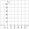
  $An empty Cartesian grid.$
  
  Figure 44. An empty grid.
🔗

Checkpoint 45. Limit, Continuity, and Differentiability.

Sort each statement to the property that it guarantees.

The graph has no break, hole, or jump at $x=a\text{.}$
$\displaystyle\lim_{x\to a}f(x)=f(a)\text{.}$
$f$ is continuous at $x=a\text{.}$
The graph is locally linear at $x=a\text{.}$
The graph has a well-defined tangent line at $x=a\text{.}$
$f$ is differentiable at $x=a\text{.}$
The left-hand limit equals the right-hand limit.
The graph approaches the same y-value from both sides.
$\displaystyle\lim_{x\to a}f(x)$ exists.
The graph has a sharp corner at $x=a\text{.}$
$f$ can be continuous but not differentiable at $x=a\text{.}$

Section After class

Solidifying the concepts discussed in class through practice is necessary to build your skills.

Watch this video which will reinforce the definition of continuity: Continuity (7:41).
Explore the following applet. This will let you practice in deciding when a function is continuous (10 examples).
Explore your understanding of continuity, removable discontinuities, and right- and left-sided limits through this applet. Read how to operate this or just move the red dot on the graph and the blue dots on the right side to mimic taking a limit graphically.
Read section 1.7.4.
Ask Copilot to “Produce a function $f(x)$ that is continuous at $x=1$ but not differentiable there and that has a limit at $x=2$ but is not continuous there.” Is the function returned to your correct?
Ask Copilot “What is the difference between a removable discontinuity and a jump discontinuity? Are there other types of discontinuities?”
Watch this video on determining differentiability graphically: Determining Differentiability Graphically (4:40).
Do Exercises 1-6 in section 1.7.6.
Read the summary in section 1.7.5.
Do Exercises 7-10 in section 1.7.6.
Explore continuity and differentiability with this applet: Continuity and Differentiability with Parameters. As always, read the paragraphs below the applet for context and understanding.
Start working on the MOMwork (MyOpenMath) assignment for this section.

Section Advanced learning objectives

In addition to mastering the basic objectives, here are the tasks you should be able to perform after class, with practice:

Provide examples (both graphically and numerically) of functions where both one-sided limits exist at a point, and yet the limit at that point fails to exist.
Determine, given an algebraic expression for a function $f\text{,}$ where it is continuous.
Describe what makes a discontinuity removable - graphically and in your own words.
Explain the relationship between continuity and differentiability.
Compute the linear approximation of a function at a specific point.

Section Additional suggestions

Watch video: Limits of a piecewise function (6:38).
Watch this video on determining when piecewise functions are continuous: Determining Continuity of a Piecewise Function (7:00).

Section Answers

🔗
🔗
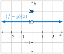
1. The graph of $(f-g)(x)$ is shown in Figure 46.
  
  $A coordinate graph showing the function labeled (f minus g)(x). The graph is a horizontal line at y equals 1 extending left and right with arrowheads. There is an open circle at the point (0, 1). Above it, a filled point is shown at (0, 2). The x- and y-axes are labeled, and the grid includes tick marks at integer values.$
  
  Figure 46. The graph of $(f-g)(x)\text{.}$
2. Yes (they are both 1).
3. Yes (they are both 1).
4. No (the limits on the left do not exist).
🔗
🔗
Notice that $2-x^{2} \leq f(x) \leq 2+x^{2}$ for all $x$ shown. Since $-1 \leq \sin\left(\frac{1}{x}\right) \leq 1$ for all $x\text{,}$ we have

\begin{gather*} -x^{2} \leq x^{2}\sin\left( \frac{1}{x}\right) \leq x^{2} \end{gather*}

so that

\begin{gather*} 2-x^{2} \leq 2+x^{2}\sin\left( \frac{1}{x}\right) \leq 2+x^{2} \end{gather*}

for all $x$ as well. Since $\lim_{x \rightarrow 0}2-x^{2} = \lim_{x \rightarrow 0}2+x^{2} = 2\text{,}$ we also then have $\lim_{x \rightarrow 0}f(x) = 2\text{.}$
Note that
- $\displaystyle \displaystyle \lim_{t \rightarrow 2^-}B(t) = \lim_{t \rightarrow 2^-}4-\frac{1}{2}t = 3$
- $\displaystyle \displaystyle \lim_{t \rightarrow 2^+}B(t) = \lim_{t \rightarrow 2^+}\sqrt{t+c}= \sqrt{2+c}$
🔗
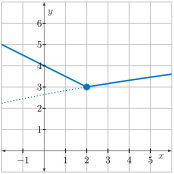
so that $\displaystyle \lim_{t \rightarrow 2}B(t)$ exists if and only if $3 = \sqrt{2+c}\text{.}$ That is, exactly when $c=7\text{.}$

$A coordinate graph showing a piecewise linear function. For x less than 2, a solid line with negative slope decreases toward the point (2, 3). At x equals 2, there is a filled point at (2, 3). For x greater than 2, a solid line with positive slope increases to the right from that point. A dotted line with smaller positive slope approaches the point (2, 3) from the left. The x- and y-axes are labeled, with a grid and integer tick marks.$

Figure 47. The graph of $B(t)\text{.}$

🔗

Prev Top Next