Handout Daily Prep 1.3 - The Derivative of a Function at a Point

Section Overview

Up next in our discussions is the definition of the foundational idea of nearly all first semester calculus: the derivative of a function at a point. As you will see soon, the derivative relies upon the ideas of average rate of change and limits. Indeed, the derivative is all about change that is happening instantaneously, and that instantaneous rate is the limit of corresponding average rates. One especially important note at the outset: the definition of the derivative is notationally complicated. As you read and study, pay close attention to the notation used in the definition of the derivative, and strive to not only know that notation by heart, but to make sense of it for yourself.
This section covers the following concepts: Average and instantaneous rate of change. Definition of the derivative at a point. Differentiability. Units of the derivative. Slope of the tangent line.

Section Basic learning objectives

These are the tasks you should be able to perform with reasonable fluency when you arrive at our next class meeting. Important new vocabulary words are indicated in italics.
  • State the definition of average rate of change and the definition of instantaneous rate of change of a function \(f\text{.}\) Explain the difference between these two quantities.
  • State the definition of the derivative of \(f(x)\) at a point \(x=a\text{.}\)
  • Illustrate the average rate of change and the instantaneous rate of change on the graph of a function.
  • Describe the derivative in terms of the slope of a tangent line.
  • Give the units of the derivative of a function, given the units of the function and of the domain variable.
  • Explain the difference between the quantities \(f(a)\) and \(f'(a)\text{.}\)

Section To prepare for class

Complete all actions listed below. Respond to the questions highlighted with Submit.
A single .pdf should be uploaded to D2L Brightspace. All answers should be briefly justified, whether justification is specifically requested or not.

Checkpoint 21. πŸ“ [Submit] Equivalent Interpretations of the Derivative.

Section After class

Solidifying the concepts discussed in class through practice is necessary to build your skills. Mathematics is not a spectator sport!

Section Advanced learning objectives

In addition to mastering the basic objectives, here are the tasks you should be able to perform after class, with practice:
  • Use the definition of the derivative to find the instantaneous rate of change of a function at a particular point.
  • Compute the equation of the tangent line to a function’s graph at a specific point.
  • Interpret the meaning of the derivative obtained from a computation in a word problem in everyday terms, using correct units.

Section Additional suggestions

  • Do these exercises.
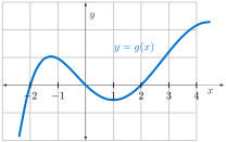
    1. For the function whose graph is given, arrange the following numbers in increasing order. Explain your reasoning.
      Graph of a function labeled y = g(x) on a coordinate grid. The horizontal axis is labeled x and the vertical axis is labeled y, with integer tick marks shown. The graph is a single smooth curve. On the far left, for x less than about βˆ’2, the graph is below the x-axis and increasing steeply. The curve rises and reaches a local maximum slightly above the x-axis near x = βˆ’1. It then decreases, crossing near the x-axis close to x = 0, and continues downward to a local minimum below the x-axis near x = 1. After this minimum, the graph increases again, crossing the x-axis near x = 2. For x greater than 2, the curve continues to rise, becoming steeper and reaching positive y-values near the right end of the graph. The curve shows no breaks, open circles, or endpoints, indicating that g is continuous over the displayed interval."
      Figure 23. The graph of \(y=g(x)\text{.}\)
      \(0 \ \ \ \ \ g'(-2) \ \ \ \ \ g'(0) \ \ \ \ \ g'(2) \ \ \ \ \ g'(4)\)
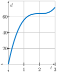
    2. A car is traveling down a highway away from its starting location with distance function \(\displaystyle d(t) = 8(t^{3} - 6t^{2} + 12t)\) where \(t\) is in hours and \(d\) is in miles.
      Graph of a function with the horizontal axis labeled t and the vertical axis labeled d, both with tick marks. The t-axis runs from 0 to about 3, and the d-axis runs from 0 to about 70. The graph is a single smooth increasing curve. Starting at t = 0, the graph begins near d = 0 and rises steeply for small values of t. As t increases toward 1, the curve continues to increase but with a decreasing slope. Between t = 1 and t = 2, the graph is nearly horizontal near d = 60, indicating very slow increase. After t = 2, the graph rises again and ends near d = 70 at t = 3. The curve has no breaks, endpoints, or open circles, indicating a continuous function over the displayed interval."
      Figure 24. The graph of \(d(t)=8(t^3-6t^2+12t)\text{.}\)
      1. How far has the car traveled after 1, 2, and 3 hours?
      2. What is the average velocity over the intervals \([0,1]\text{,}\) \([1,2]\text{,}\) and \([2,3]\text{?}\)
      3. The graph of \(d(t)\) on \([0,3]\) is given.
        1. Does the car ever stop?
        2. What is the average velocity over \([1,3]\text{?}\) over \([1.5,2.5]\text{?}\) over \([1.9,2.1]\text{?}\)
      4. Estimate the instantaneous velocity at \(t=2\text{.}\) Give a physical interpretation of your answer.
    3. Find a function \(f\) and a number \(a\) such that
      1. \(\displaystyle \displaystyle \lim_{h \rightarrow 0}\frac{(2+h)^{5} - 32}{h}= f'(a)\)
      2. \(\displaystyle \displaystyle \lim_{h \rightarrow 0}\frac{[(-1+h)^{3}-(-1+h)]-[(-1)^{3}-(-1)]}{h}= f'(a)\)
      1. If \(f\) is an even function and \(f'(4) = 5\text{,}\) what is \(f'(-4)\text{?}\)
      2. If \(g\) is an odd function and \(g'(10) = 6\text{,}\) what is \(g'(-10)\text{?}\)
      3. If \(f\) is any even function, and \(f'(0)\) exists, what is \(f'(0)\text{?}\) Why?
      4. If \(f\) is an odd function, what (if anything) can be said about \(f'(0)\text{?}\)

Section Answers

Subsection To prepare for class

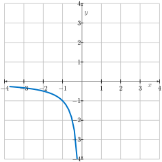
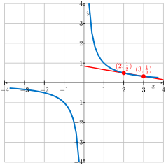
    1. The full graph of \(f\) is shown in FigureΒ 25.
      Graph of a function on a coordinate grid with the horizontal axis labeled x and the vertical axis labeled y, both marked with integer tick marks. The graph consists of two separate smooth curves and a secant line. One curve appears in the lower-left portion of the graph, for x less than about βˆ’1. This curve decreases as x increases, crossing near y = 0 around x = βˆ’3 and then falling rapidly, becoming very steep as it approaches x = 0 from the left. A second curve appears in the upper right portion of the graph, for x greater than about 1. This curve begins at high positive y-values just to the right of x = 1 and decreases as x increases. It passes near the points (2, 1) and (3, 0.5), which are shown as filled points and labeled accordingly. A red line segment is drawn connecting the points (2, 1) and (3, 0.5). This secant line slopes downward from left to right and intersects the graph only at these two labeled points. There is a gap between the two curves near x = 0, indicating the function is not defined or not shown there. The figure emphasizes the use of two points on the graph to form a secant line."
      Figure 25. The graph of \(f(x)=2^x\) together with a secant line through \((2,f(2))\) and \((3,f(3))\text{.}\)
    2. The secant line through \((2,f(2))\) and \((3,f(3))\) is shown in red in FigureΒ 25.
    3. \(\displaystyle \displaystyle \frac{-1}{2(2+h)}\)
    4. The apparent slope is -1/4.
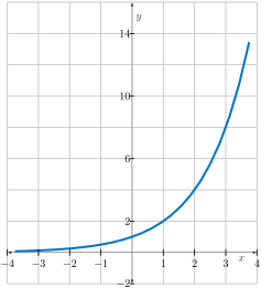
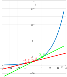
  1. The graph of \(g(x) = 2^{x}\) with secant and tangent lines appears in FigureΒ 26.
    Graph of a function on a coordinate grid with the horizontal axis labeled x and the vertical axis labeled y, both marked with integer tick marks. The graph shows a smooth increasing curve that passes near the x-axis on the left and rises steeply for x greater than about 1, reaching large y-values by x = 4. Two points on the curve are highlighted and labeled. One point is labeled (βˆ’1, one-half), and another is labeled (1, 2). A straight line is drawn through each of these points, representing tangent or linear approximation lines. The line through the point (βˆ’1, one-half) has a shallow positive slope and extends across the graph. The line through the point (1, 2) has a steeper positive slope and intersects the curve near that point. At the point (0, 1), the curve passes through the y-axis and is shown to lie between the two straight lines. The figure illustrates how the slopes of the tangent lines differ at different points on the curve and how the function’s rate of change increases as x increases."
    Figure 26. The graph of \(f(x)=2^x\) with secant and tangent lines.
    1. The secant line through \((-1,g(-1))\) and \((0,g(0))\) is shown in red in FigureΒ 26..
    2. An equation for the secant line is \(y=x+1\text{.}\) It is shown as a green line in FigureΒ 26.
    3. Based on your results above, we can say about the slope of the tangent line to \(g(x)\) at \(x=0\) has a slope between \(\frac{1}{2}\) and 1.
    4. As \(h\) approaches 0, we would guess that the slope of the tangent line approaches \(\ln 2 \approx 0.69\text{.}\) [Later, we will see it is exactly \(\ln 2\text{.}\) For now, we estimate 0.7 or so.]

Subsection After class

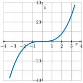
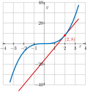
  1. The equation of the tangent line to \(y=x^{3}\) at \(x=2\) is \(y=12x-16\text{.}\) A sketch of this tangent line on the curve is shown in FigureΒ 27 in red. To find this line, note that the slope of this line is \(\displaystyle \lim_{h \rightarrow 0}\frac{(2+h)^{3}-2^{3}}{h}= 12\text{.}\) Then, recognize that \((2,8)\) is a point on the line so that \(y-8 = 12(x-2)\) represents the line.

    Graph of a function on a coordinate grid with the horizontal axis labeled x and the vertical axis labeled y, both marked with integer tick marks from approximately βˆ’4 to 4 on the x-axis and βˆ’40 to 40 on the y-axis. The graph shows a single smooth increasing curve with an S-shaped appearance. On the left, for x near βˆ’4, the curve is well below the x-axis and increasing. As x increases toward βˆ’1, the graph flattens slightly near the x-axis, then continues upward. For x greater than about 1, the curve increases rapidly, becoming steep near the right edge of the graph. A straight line is drawn that intersects the curve at a marked point labeled (2, 8). This line has positive slope and passes through the point (2, 8), extending downward to the left and upward to the right. The line is steeper than the curve for x less than 2 and less steep than the curve for x greater than 2. The figure illustrates a tangent or linear approximation to the curve at the point (2, 8), highlighting the local behavior of the function near that point."
    Figure 27. The graph of the tangent line to \(y=x^3\) at \(x=2\) is \(y=12x-16\text{.}\)

Subsection Additional suggestions

  1. \(\displaystyle g'(0) < 0 < g'(4) < g'(2) < g'(-2)\)
    1. \(d(1)=56\) miles, \(d(2) = 64\) miles, \(d(3) = 72\) miles
    2. \(\displaystyle AV_{[0,1]}= \frac{d(1)-d(0)}{1-0}= 56\) mph, \(\displaystyle AV_{[1,2]}= \frac{d(2)-d(1)}{2-1}= 8\) mph, \(\displaystyle AV_{[2,3]}= \frac{d(3)-d(2)}{3-2}= 8\) mph
      1. Yes, it stops at time \(t=2\) (hours).
      2. \(\displaystyle AV_{[1,3]}= \frac{d(3)-d(1)}{3-1}= 8\) mph, \(\displaystyle AV_{[1.5,2.5]}= \frac{d(2.5)-d(1.5)}{2.5-1.5}= 2\) mph, \(\displaystyle AV_{[1.9,2.1]}= \frac{d(2.1)-d(1.9)}{2.1-1.9}= 0.08\) mph
    3. We estimate the instantaneous velocity at \(t=2\) hours to be 0 mph (stopped).
    1. \(f(x) = x^{5}\) where \(a=5\)
    2. \(f(x) = x^{3}-x\) where \(a=-1\)