Our main focus in this section will be on understanding how calculus ideas can be used to answer the question of “where is a given function greatest or least?” We will begin with a more theoretical discussion of optimization, learning about the Extreme Value Theorem, and from there we’ll proceed to more applied settings where we see how calculus provides rigorous answers to interesting questions.
These are the tasks you should be able to perform with reasonable fluency when you arrive at our next class meeting. Important new vocabulary words are indicated in italics.
State the Extreme Value Theorem and enumerate the multi-stage process used for finding the global/absolute extreme values of a function on a closed, bounded interval.
📝 [Submit] Explore applet Absolute Max and Min. Then, submit three screen captures - (1) showing the function on some closed interval \([a,b]\) for which the absolute maximum and absolute minimum are located in the open interval \((a,b)\text{,}\) (2) showing the function on some closed interval \([a,b]\) for which the absolute maximum is located at an endpoint and the absolute minimum is located in the open interval \((a,b)\text{,}\) and (3) showing the function on some closed interval \([a,b]\) for which the absolute maximum and absolute minimum are both located at endpoints.
📝 [Submit] Find the absolute maximum and absolute minimum of \(\displaystyle f(x) = x^{2} - 3x^{\frac{2}{3}}\) over interval \([0,2]\) and state where those values occur.
Prompt Copilot “Find the absolute maximum and absolute minimum of f(x) = x\(\wedge\)2 - 3x\(\wedge\)(2/3) over interval [0,2] and state where those values occur.” Follow up with “Explain why you came to the conclusion you did.” Does the AI get this correct?
In each optimization problem, one quantity is the objective: the quantity that must be made as large or as small as possible. Match each situation with its objective function.
A farmer has a fixed amount of fencing and wants to enclose the largest possible rectangular pasture.
Maximize the area: \(A=xy\text{.}\)
A soup company wants a cylindrical can that holds a fixed volume using the least material.
Minimize the surface area: \(S=2\pi r^2+2\pi rh\text{.}\)
A manufacturer wants to build an open-top box from a rectangular sheet of cardboard by cutting equal squares from the corners. The box should hold as much as possible.
Explore this applet Optimization - Function and Rectangle 1 and determine an answer to the question posed by using calculus. The following may help guide you.
List the critical points of \(A(x)\) and endpoints of the interval on which you are seeking to maximize \(A(x)\text{.}\) Which of these values will produce the largest output? How do you know?
Explore this second (related) applet Optimization - Function and Rectangle 2 and determine an answer to the question posed by using calculus. The following may help guide you.
List the critical points of \(A(x)\) and endpoints of the interval on which you are seeking to maximize \(A(x)\text{.}\) Which of these values will produce the largest output? How do you know?
Prompt Copilot “Find the absolute maximum and absolute minimum of p(x) = x\(\wedge\)3 - a\(\wedge\)2*x on the interval [0,a] for a>0.” Compare the answer you receive with that of Exercise 8a in section 3.5.5 in the text. Is the AI correct?
Explore this version of a figure giving The Extreme Value Theorem Visualization. Nothing to move here - just a picture and a statement you want to internalize.
Watch this video Extrema on a Closed Interval (7:48) if you are interested in seeing another example of the maximization process on a closed, bounded interval.
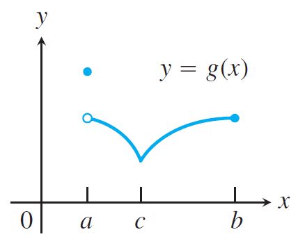
The absolute minimum occurs at \(x=c\text{.}\) The absolute maximum occurs at \(x=a\text{.}\) The Extreme Value Theorem does not apply to this case since the function is not continuous on the interval \([a,b]\text{.}\) So the existence (or not) of absolute extrema is not guaranteed. However, that doesn’t mean, of course, that it cannot happen. In this case, it does.
First, we evaluate \(f\) at the endpoints \(x=0\) and \(x=2\text{.}\) Note that \(f(0)=0\) and \(f(2) = 4-3(2)^{2/3}\approx -0.762\text{.}\) Then, we compute \(f'(x)\text{.}\)
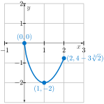
for \(x \neq 0\text{.}\) We see that \(f'(x)=0\) when \(2x^{4/3}-2=0\) which implies that \(x=\pm 1\text{.}\) The derivative does not exist when \(x=0\text{.}\) So the critical points of \(f\) are at \(x=-1,0,1\text{.}\) Since \(x=0\) is an endpoint of the interval \([0,2]\text{,}\) we have already evaluated it. Since \(x=-1\) is not in the interval of interest, we need only evaluate \(f(1)\text{.}\) We find \(f(1)=-2\) . We then compare the values found: \(f(0)=0, f(1) = -2\text{,}\) and \(f(2)\approx -0.762\text{.}\) By the Extreme Value Theorem, we know the global minimum is -2 and occurs at \(x=1\text{.}\) We also know the absolute maximum is 0 and occurs at \(x=0\text{.}\) A sketch of the graph on \([0,2]\) appears below.