In this section, we once again address the question of how to construct the graph of \(f(x)\) if we know the graph of its derivative \(f'(x)\text{.}\) We also take a look at functions defined as a definite integral with a variable as a limit of integration, and see how this is a type of function that we can analyze.
These are the tasks you should be able to perform with reasonable fluency when you arrive at our next class meeting. Important new vocabulary words are indicated in italics.
Evaluate integral functions such as \(\displaystyle A(x) = \int_{0}^{x} g(t) \ dt\) at various \(x\) values when given a simple formula or graph for \(g(t)\text{.}\)
Explore the applet Identify an Antiderivative Function to use cues given in the graph of a function in construction of an antiderivative of it. Practice as you wish.
📝 [Submit] Readsection 5.1.3. For the situation presented in Figure 5.1.3, it is said that “Similarly, \(F(2)=1.5, F(3)=-0.5, F(4)=-2\text{,}\)\(F(5)=-0.5\text{,}\) and \(F(6)=1\text{.}\) Explain how it is that \(F(2)=1.5\) and \(F(3)=-0.5\text{.}\)
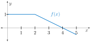
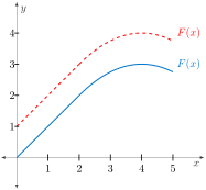
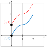
Sketch two functions \(F\) such that \(F' = f\text{.}\) In one case, let \(F(0)=0\) and in the other let \(F(0)=1\text{.}\)Figure 132 gives a graph of \(f(x)\text{.}\)
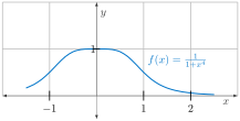
📝 [Submit] Graph an antiderivative \(F\) of \(\displaystyle f(x) = \frac{1}{1+x^{4}}\) for which \(F(-1) = 0\text{.}\) Discuss maxima, minima, concavity, and intervals of increase/decrease.
Prompt Copilot “How can I use the concept of signed area under a curve to plot the antiderivative of a given graph of a function?” Follow the response you receive with the prompt “Can you repeat this but use integral signs to help me understand how definite integrals play a role in this process?”
Prompt Copilot “If a function \(f(x)\) is positive, decreasing, and concave up, what graphical properties should I expect an antiderivative to have?” You may get a response with the phrase horizontal inflection point. What is that?
Explore the applet Area Function. The default blue function \(f\) is obviously \(f(t)=t^{2}\text{.}\) The red dotted function is \(\displaystyle F(x) = \int_{L}^{a} f(t) \ dt\) where \(a\) is determined by the slider. What is the value of this lower limit \(L\text{?}\)
Explore the applet Area Function. For the default function \(f(t)=(t-1)^{2}-4\) given, change the value of \(a\) to 1. Does it make sense that \(F(x)\) has a local max at -1 and a local min at 3? What about the graph of \(f(t)\) tells you that might happen?
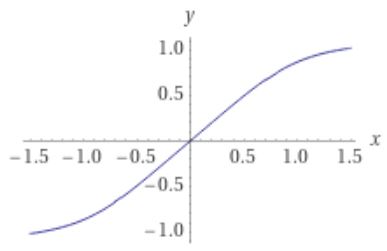
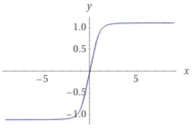
If \(F'(x)=f(x)\text{,}\) then note that \(F\) is always increasing since \(F'(x) > 0\) always holds. Hence, there is no maximum or minimum. Since \(f' > 0\) on \((-\infty,0)\) and \(f'<0\) on \((0,\infty)\text{,}\) we have that the same is true for \(F''\text{.}\) So, \(F\) is concave up on \((-\infty,0)\) and concave down on \((0,\infty)\text{.}\) Knowing the graph of \(F\) goes through the point \((-1,0)\) gives a good sense of how \(F\) behaves. Figure 137 shows two different views of \(F(x)\text{.}\)