The derivative of a function tells us key information. We now investigate the concept of optimization. That is, we are interested in determining where the value of a function is greatest or least, and the input value(s) at which such extremes occur. As we move from Section 3.5 into Section 3.6, we start to emphasize problems that occur in a more applied setting, ones that are based in some sort of physical reality. Here, you will be challenged to read carefully and interpret different possible scenarios, identify variables and determine functions, and to use calculus to justify the reasoning behind your ultimate answers.
These are the tasks you should be able to perform with reasonable fluency when you arrive at our next class meeting. Important new vocabulary words are indicated in italics.
Use a constraint in the problem to reduce the number of other variables in the equation to one, and solve for the target quantity to obtain a function of one variable.
After completion, look back by using GeoGebra to graph the function \(f(x) = x^{2}(108-4x)\) on \([0,27]\text{.}\) How does this graph relate to your solution to the problem?
📝 [Submit] If you have 100 feet of fencing and want to enclose a rectangular area up against a long, straight wall, what is the largest area you can enclose?
Prompt Copilot “If you have 100 feet of fencing and want to enclose a rectangular area up against a long, straight wall, what is the largest area you can enclose? Explain.” Does the AI get this question correct? Does it even use calculus to ‘solve’ the problem?
Prompt Copilot “Find a positive number such that the sum of the number and twice its reciprocal is as small as possible. Explain.” Follow up the response by prompting “But just because the derivative is 0 does not make this value a minimum. So why do you claim it is?” Does the AI give useful and correct feedback?
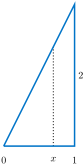
Hint: The function \(A(x)\) you seek to maximize on domain \([0,1]\) is the product of the area of the “smaller” triangle and what remains. The area of what remains is simply the area of the large triangle minus the area of the small triangle.
If you would like a hint, Khan Academy as a video you can watch that explains how to do a similar problem (though without GeoGebra and with different dimensions given. See Optimization: Box Volume (Part I) and Optimization: Box Volume (Part II). He makes mistakes (such as not using an approximation symbol when he should), but the solution process is reasonable.
In each optimization problem, one variable has already been eliminated using the given constraint. Match the situation with the correct one-variable objective function that should be optimized.
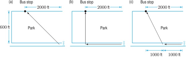
Alaina wants to get to the bus stop as quickly as possible. The bus stop is across a grassy park, 2000 feet west and 600 feet north of her current position. Alaina can walk west along the edge of the park on the sidewalk at a speed of 6 ft/sec. She can also travel through the grass in the park, but only at a rate of 4 ft/sec.
Of the paths shown in the diagram above, the one in (a) is the shortest in length and the one in (b) is the longest in length. Which one of these three is the shortest in time?
If Alaina walks \(x\) feet west along the sidewalk before heading diagonally across the park to the bus stop, the total time it takes her will be \(T = T_{sidewalk}+ T_{park}\text{.}\) Write \(T\) as a function of \(x\text{.}\)
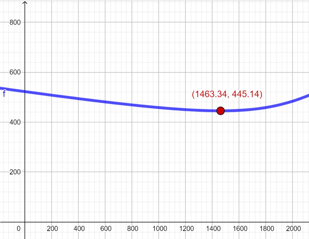
What is the domain of the function \(T\) found in part (b)? For what value of \(x\) on this domain is this function minimized? What is the minimum value? GeoGebra may be used to help estimate this value.
In a wide range of contexts, identify and formulate a function of interest and then use calculus to accurately justify where the function is optimized on an appropriate domain.
Our goal is to maximize \(A(x,y) = xy\) where \(x\) represents the length of two sides of fence and \(y\) is the length of the other (the length parallel to the wall being used). We maximize \(A(x,y)\) subject to the condition that \(2x+y=100\text{.}\) By solving for \(y\text{,}\) we aim to maximize
on the domain \(0 \leq x \leq 50\) (because \(0 \leq y=100-2x \leq 100\)). Since \(A'(x) = 100-4x\) we find a critical value at \(x=25\) that leads to a global maximum of \(A\) on its domain. \(A(25) = 1250\text{.}\)
The positive number is \(\sqrt{2}\text{.}\) The function \(Q(x)\) being minimized is \(Q(x) = x + \frac{2}{x}\text{.}\) It is being minimized on the domain \((0,\infty)\text{.}\) Since \(Q'(x) = 1-2x^{-2}= 1-\frac{2}{x^{2}}= 0\) exactly when \(x=\pm \sqrt{2}\text{,}\) we see that \(\sqrt{2}\) is the only critical point in the domain. A first derivative sign chart shows us that this is a local minimum.
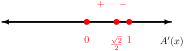
It follows that \(A'(x)=0\) exactly when \(x=0\) or \(\displaystyle x=\pm \frac{\sqrt{2}}{2}\text{.}\) A first derivative sign chart appears in Figure 95.
In (c), the distance is \(1000 + \sqrt{1000^{2} + 600^{2}}\approx 2166\) feet. It takes \(1000/6 + 1166/4 \approx 458\) seconds. This is the shortest time.