Handout Daily Prep 1.1 - Average Velocity

Section Overview

This section discusses the following concepts: Average velocity. Slope of a secant line. Instantaneous velocity.

Section Basic learning objectives

These are the tasks you should be able to perform with reasonable fluency when you arrive at our next class meeting. Important new vocabulary words are indicated in italics.
  • Determine the position of an object at a specific time given a position function for the object.
  • Compute the average velocity of an object on a specific time interval.
  • State the units of the average velocity of an object.

Section To prepare for class

Complete all actions listed below. Respond to the questions highlighted with Submit.
A single .pdf should be uploaded to D2L Brightspace. See the syllabus for grading rubric. It is not necessary to re-state the questions. Instead, simply enumerate your responses clearly. Strive to use valid notation and correct mathematical language and syntax. All answers should be briefly justified, whether justification is specifically requested or not.

Checkpoint 8. Representations of Average Velocity.

Section After class

Solidifying the concepts discussed in class through practice is necessary to build your skills. Mathematics is not a spectator sport!
  • Prompt Copilot β€œUse mathematical notation to give the precise relationship between instantaneous velocity and average velocity.”
  • Prompt Copilot β€œHow is delta notation used in calculus?”
  • Do the following exercise.
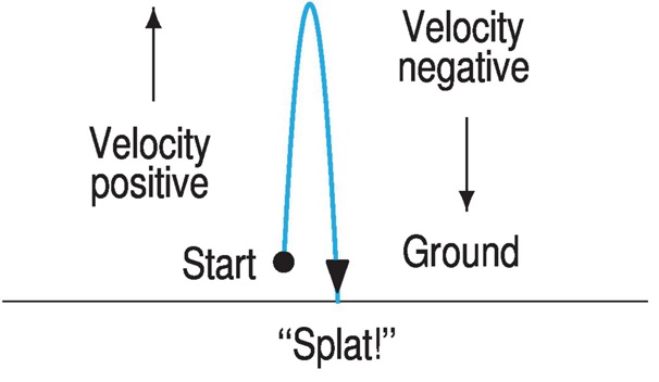
    1. We look at the speed of a grapefruit that is thrown straight upward into the air at \(t=0\) seconds.
      A curve showing the height of a grapefruit over time.  The curve increases, reaches a peak, and then decreases.
      Figure 9. Height of a grapefruit over time.
      The grapefruit leaves the thrower’s hand at high speed, slows down until it reaches its maximum height, and then speeds up in the downward direction and finally, β€œSplat!”.
      Table 10. Height of the grapefruit above the ground.
      \(t\) (sec) 0 1 2 3 4 5 6
      \(y\) (feet) 6 90 142 162 150 106 30
      1. Did the grapefruit travel faster over the first interval \(0 \leq t \leq 1\) or the second interval \(1 \leq t \leq 2\text{?}\)
      2. Compute the average velocity of the grapefruit over the interval \(4 \leq t \leq 5\text{.}\) What is the significance of the sign of your answer?
      3. The grapefruit traveled faster over the first interval \(0 \leq t \leq 1\) than the second interval \(1 \leq t \leq 2\text{.}\) If the data in the table can be modeled by \(y=6+100t-16t^{2}\text{,}\) fill in the table below to estimate the value of the instantaneous velocity at time \(t=1\) second. Then, give an expression for the average velocity \(AV_{[a,a+h]}\) of the grapefruit on the time interval \([a,a+h]\text{.}\)
        Table 11. Average velocity of the grapefruit over various time intervals.
        Time Interval Average Velocity
        [1,1.5]
        [1,1.1]
        [1,1.01]
        [1,1.001]
        [1,1.0001]
        [0.999,1]
        [0.9999,1]
  • Do exercises 1-8 in section 1.1.5 of the text. These are interactive WebWork exercises intended to give you instantaneous feedback.
  • Read summary in Section 1.1.4.
  • Start working on the MOMwork (MyOpenMath) assignment for this section.

Section Advanced learning objectives

In addition to mastering the basic objectives, here are the tasks you should be able to perform after class, with practice:
  • Interpret average velocity graphically.
  • Differentiate between instantaneous velocity and average velocity.
  • Determine the average velocity of an object on an interval starting at time \(t=a\) and ending at time \(t=a+h\text{,}\) where \(a\) is given but \(h\) is a variable. Express the result in simplest form as a function of \(h\text{.}\)
  • Determine the instantaneous velocity at the single moment \(t=a\) given the average velocity of an object from time \(t=a\) to time \(t=a+h\text{.}\)

Section Additional suggestions

Section Answers

Subsection To prepare for class

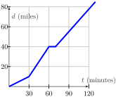
    1. Don’t confuse Katherine’s distance with her velocity.
      Graph of distance d, measured in miles, as a function of time t, measured in minutes. The horizontal axis is labeled t in minutes and runs from 0 to 120. The vertical axis is labeled d in miles and shows values from 0 to about 80. The graph is piecewise linear. From t equals 0 to t equals 30, the distance increases slowly from 0 to about 10 miles. From t equals 30 to t equals 60, the distance increases more rapidly, reaching 40 miles at t equals 60. From t equals 60 to t equals 75, the graph is horizontal at d equals 40, indicating that the distance does not change during this time interval. From t equals 75 to t equals 120, the distance increases again at a steady rate, ending near 80 miles at t equals 120. Changes in slope indicate changes in speed, and the horizontal segment indicates a period of no motion.
      Figure 12. Katherine’s distance vs. time.
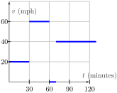
    2. Graph of velocity v, measured in miles per hour, as a function of time t, measured in minutes. The horizontal axis is labeled t in minutes and runs from 0 to 120. The vertical axis is labeled v in miles per hour and shows values from 0 to about 70. The graph is piecewise constant and consists of horizontal line segments. From t equals 0 to t equals 30, the velocity is constant at 20 miles per hour. From t equals 30 to t equals 60, the velocity jumps to 60 miles per hour and remains constant. At t equals 60, the velocity drops abruptly to zero for a short interval. From about t equals 70 to t equals 120, the velocity is constant again at 40 miles per hour. The vertical jumps between segments indicate instantaneous changes in velocity, and there are no sloped segments shown.
      Figure 13. Katherine’s velocity vs. time.
    3. Katherine’s average speed is \(\displaystyle v = \frac{85 \ {miles}}{130 \ {min}}\cdot \frac{60 \ {min}}{1 \ {hr}}\approx 39.23\) mph.
  1. Velocity is distance divided by time. That is, \(\displaystyle v = \frac{d}{t}\text{.}\)
    For the first leg of her trip, the time taken is \(t_{1} = 0.75\) hours.
    For the second leg of her trip, the distance traveled is \(d_{2} = 30\) miles.
    This information is useful in computing the total distance and the total time for the whole trip. The total distance is 30 + 30 or 60 miles. The total time taken is 0.75 + 0.5 = 1.25 hours.
    So, her average velocity is \(v = \frac{60 \ {miles}}{1.25 \ {hour}}= 48\) mph.
  2. The first leg of Dale’s trip is 20 miles. The second leg of Dale’s trip is 30 miles.
    So, the average velocity on his trip is \(v = \frac{50 \ {miles}}{1 \ {hour}}= 50\) mph.
  3. In order to average 60 mph for the entire trip, the total time taken should be \(\displaystyle t = \frac{2 \ {miles}}{60 \ {mph}}= \frac{1}{30}\) or 2 minutes.
    But, the first leg of the trip takes \(\displaystyle t = \frac{1 \ {mile}}{30 \ {mph}}=\) 2 minutes. So it is impossible to average this velocity since it will take a positive amount of time to travel the second mile.

Subsection After class

    1. The velocity on \(0 \leq t \leq 1\) is \(\displaystyle \frac{\Delta y}{\Delta t}= \frac{90-6}{1-0}= 84\) ft/sec.
      The velocity on \(1 \leq t \leq 2\) is \(\displaystyle \frac{\Delta y}{\Delta t}= \frac{142-90}{2-1}= 52\) ft/sec.
      The grapefruit traveled faster over the time interval \(0 \leq t \leq 1\text{.}\)
    2. The average velocity on \([4,5]\) is \(\displaystyle \frac{\Delta y}{\Delta t}= \frac{106-150}{5-4}= -44\) ft/sec. The negative sign tells us the grapefruit is traveling downward.

    3. The instantaneous velocity at time \(t=1\) is approximately 68 ft/sec.
      Table 14. Average velocities of the grapefruit on various intervals computed.
      Time Interval Average Velocity
      [1,1.5] 60 ft/sec
      [1,1.1] 66.4 ft/sec
      [1,1.01] 67.84 ft/sec
      [1,1.001] 67.984 ft/sec
      [1,1.0001] 67.9984 ft/sec
      [0.999,1] 68.016 ft/sec
      [0.9999,1] 68.0016 ft/sec