The theme of this chapter centers on what we can learn from key information regarding the derivative of a function. In Section 3.3, we focus on how the derivative detects extreme values of functions. That is, we investigate how information from the derivative function can tell us whether the original function has a relative maximum or relative minimum at a given point. While many of the ideas in this section will be natural and intuitive (and ones we’ve discussed briefly to some extent earlier in the course), there is considerable new language and reasoning to learn and understand.
These are the tasks you should be able to perform with reasonable fluency when you arrive at our next class meeting. Important new vocabulary words are indicated in italics.
State and apply the following fact: If the function \(f\) has a local extremum at \(x=c\text{,}\) then \(c\) is a critical number of \(f\text{.}\) Be able to give examples demonstrating that the opposite is false: If \(c\) is a critical number of \(f\text{,}\) then there is not necessarily a local extremum at \(c\text{.}\)
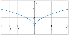
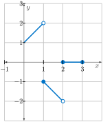
Plot the graph of \(f(x) = \sqrt{|x|}\) on each of the following domains. Then, determine if the function has a global maximum and a global minimum on that domain. Feel free to use GeoGebra to verify your thinking.
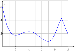
The graph of a continuous function \(f\) is given in Figure 82. Estimate the location of all relative and global maxima and minima on the domain \([0,10]\text{.}\) What do you notice about the derivative of \(f\) at these locations?
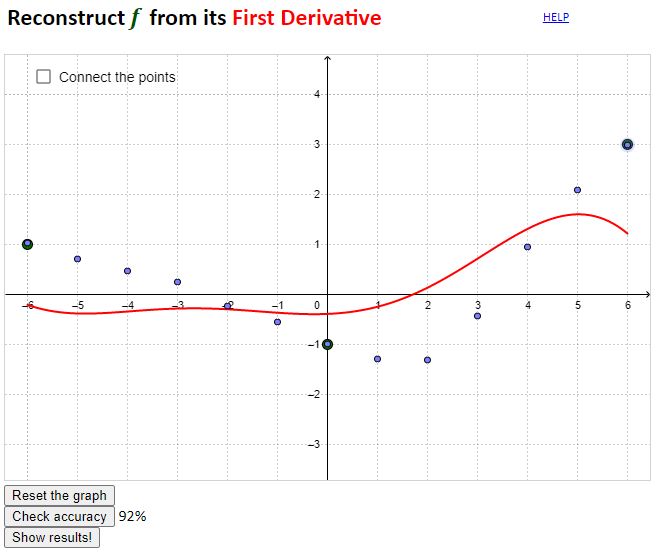
📝 [Submit] Explore applet Critical Values. Then determine the critical values for the given function in the applet. What is the behavior of \(f'(x)\) on the left and the right of these critical values? Does that behavior tell you if the critical value is a local maximum or local minimum? Explain.
Watch video Using the First Derivative Test (11:08). This video shows how to apply the First Derivative Test in practice, by using the sign table of the derivative to determine the intervals of increasing/decreasing behavior of a function.
Suppose that \(c\) is a critical number of a function \(f\text{.}\) Match each sign pattern for \(f'(x)\) with the correct conclusion about \(f\) at \(x=c\text{.}\)
Construct a sign chart for the first derivative. Use it to determine the intervals of the increasing/decreasing behavior, as well as the location of extreme values of a function.
Construct a sign chart for the second derivative. Use it to determine the intervals of the concave up/concave down behavior, as well as the location of inflection points of a function.
Use sign charts for the first and second derivative to sketch the graph of a function. (Construct sign charts for functions to find where they are increasing and decreasing, and concave up or concave down, and consequently to find extreme values and inflection points.)
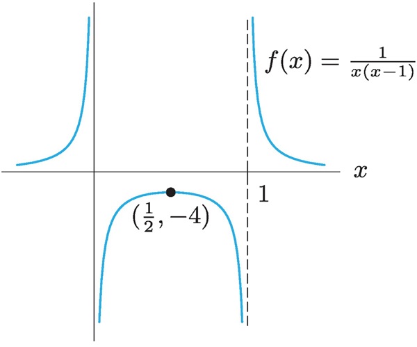
Use a graph of the function \(\displaystyle f(x) = \frac{1}{x(x-1)}\) to observe its relative maxima and minima. Verify your observation using the First Derivative Test and a sign chart.
\(f\) has local minima at \(x=2\) and \(x=7\) and local maxima at \(x=4\) and \(x=9\text{.}\)\(f\) has global minimum at \(x=7\) and global maximum at \(x=0\text{.}\) The derivative of \(f\) at local extrema is either zero or does not exist.
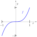
Graphically, \(f\) has a critical value at \(x=0\) (slope is zero there). Algebraically, since \(f'(x)=3x^{2}=0\) when \(x=0\text{,}\) we see that \(f\) has a critical value there. There is no maximum or minimum at \(x=0\) since the function is clearly increasing both to the left and to the right.
\(g'(t) = ae^{t} - be^{-t}= e^{-t}(ae^{2t}-b) = 0\) if and only if \(ae^{2t}=b\text{.}\) That happens exactly when \(\displaystyle e^{2t}=\frac{b}{a}\) or \(\displaystyle 2t = \ln \left( \frac{b}{a}\right)\text{.}\) Thus, the only critical value is \(\displaystyle t=\frac{1}{2}\ln \left( \frac{b}{a}\right)\text{.}\)
The graph of \(f\) suggests a local maximum exists at \(x=\frac{1}{2}\) and is a value of \(-4\text{.}\) Algebraically, \(\displaystyle f'(x) = \frac{-(2x-1)}{x(x-1)}= 0\) exactly when \(x=\frac{1}{2}\text{.}\) The sign chart below verifies that we have a local maximum at \(x=\frac{1}{2}\text{.}\)