Having now completed Chapter 1 on the definition and meaning of the derivative, we turn to Chapter 2 where our principal focus will be on computing derivatives. By this we mean that we want to further understand the limit definition of the derivative and patterns that can be found in certain classes of functions, patterns that will enable us to simply look at the formula for a function and then be able to write down a formula for the derivative. As we progress through Chapter 2, you’ll see that we will build from the simplest functions to much more complicated ones.
This section covers the following concepts: Notations for derivatives. The Power Rule. Differentiation of exponential functions. The derivative of constant multiples, sums, and differences of functions.
These are the tasks you should be able to perform with reasonable fluency when you arrive at our next class meeting. Important new vocabulary words are indicated in italics.
New Activity 2.1.1 Start by loading the applet https://www.geogebra.org/m/qwdxbtGF. Functions of the form \(f(x) = x^{n}\text{,}\) where \(n = 1, 2, 3, \ldots\) are called power functions. The first two questions below revisit work we did earlier in Chapter 1, and the following questions extend those ideas to higher powers of \(x\text{.}\)
Make a conjecture regarding a formula for the derivative of \(f(x)=x^{n}\) that holds for every positive integer \(n\text{.}\) That is, given \(f(x) = x^{n}\) where \(n\) is a positive integer, what do you think is a formula for \(f'(x)\text{?}\)
📝 [Submit] Extend your conjecture in part (d) of New Activity 2.1.1 to negative powers \(n\text{.}\) That is, using \(n = -1, -2, -3, \ldots\text{,}\) do you spot a pattern for a formula representing \(f'(x)\) if \(f(x) = x^{n}\text{?}\)
Do the following construction in GeoGebra (Google search “GeoGebra Classic” to use this tool if the link fails.). Submit screenshots and responses to the questions posed.
A slider should be created underneath. You will want to change the minimum and maximum values to 1.1 and 5.0 by clicking on these values at the left and right of the slider. Set your step size to 0.01.
In the next input box, type \(a^{x}\text{.}\) You will need to use the key above the 6. The function \(f(x)=a^{x}\) will automatically be defined, graphed, and labeled for you.
Next, you will want to use the menu. On the fourth button (see Figure 52), choose the Tangents option. Then, click on point A on your graph followed by clicking on the graph itself. This will produce a tangent line to your function \(f(x) = a^{x}\) at \((0,1)\text{.}\) It will name this tangent line \(g\) and an expression for it will appear in the next input box.
Type ln(a) in the next open input box. Move the slider and compare the slope of \(g\) to this value. What do you notice? Does this surprise you or not? Explain.
Explore the concept of derivative of polynomial functions. This applet on polynomials and derivatives, has a slider that will show the \(d\)th derivative of a 6th degree polynomial.
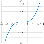
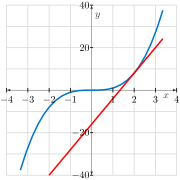
Graph the tangent line and the function on the same axes. If the tangent line is used to estimate values of the function, will the estimates be overestimates or underestimates?
\(\displaystyle \frac{dy}{dx}= 3x^{2} - 18x -16\text{.}\) So, the slope is 5 when \(3x^{2} - 18x -16=5\) or \(3x^{2} - 18x - 21=0\) . Solving \(x^{2} - 6x-7=0\) or \((x-7)(x+1)=0\) gives \(x=7\) or \(x=-1\text{.}\) The coordinates of these two points are thus \((-1,7)\) and \((7,-209)\text{.}\)